Algorithm Variants

The framework implements several optimizations to the base Seldonian algorithm [Thomas2019] that tighten confidence bounds, leading to improved solution rates and objective performance. Each variant can be selected via the seldonian_type argument.

Mode	Name	Key Idea
base	Baseline QSA	Uniform \(\delta/2\) splitting, standard Hoeffding bound
mod	Modified Confidence Interval	Decomposes candidate and safety estimation error
const	Constant-Aware Allocation	Skips delta splitting for constant nodes
bound	Union Bound Optimization	Combines delta for repeated leaf nodes
opt	All Optimizations	Combines mod, const, and bound

Baseline QSA (base)

The baseline algorithm uses uniform delta splitting and the standard Hoeffding bound [Hoeffding1963] for predicting the safety test outcome during candidate selection.

Predicted confidence interval. During candidate selection, the upper bound on \(g(\theta)\) is estimated as:

\[\hat{p} \pm 2\sqrt{\frac{\ln(1/\delta)}{2\,|\mathcal{D}_s|}}\]

where \(|\mathcal{D}_s| = (1 - r) \cdot |\mathcal{D}|\) and \(r\) is the candidate ratio.

Delta splitting. At each binary operator in the constraint expression tree, \(\delta\) is split uniformly:

\[\delta_{\text{left}} = \delta_{\text{right}} = \frac{\delta}{2}\]

uv run python -m fair_seldonian.experiments.runner base

Modified Confidence Interval (mod)

The baseline doubles the Hoeffding term to account for estimation error in both the candidate estimate and the safety bound. This is conservative: the two sources of error have different sample sizes.

The modified bound decomposes the interval into separate terms:

\[\hat{p} \pm \underbrace{\sqrt{\frac{\ln(1/\delta)}{2\,|\mathcal{D}_c|}}}_{\text{candidate error}} + \underbrace{\sqrt{\frac{\ln(1/\delta)}{2\,|\mathcal{D}_s|}}}_{\text{safety error}}\]

When does this help? When \(|\mathcal{D}_c| \neq |\mathcal{D}_s|\), the decomposed form yields a tighter interval than doubling the safety-only term. The improvement is most pronounced at extreme candidate ratios.

uv run python -m fair_seldonian.experiments.runner mod

Constant-Aware Delta Allocation (const)

In the baseline, delta is split equally at every binary operator node. However, when one child is a numeric constant (e.g., 0.25), its value is exact — no confidence interval is needed. The full \(\delta\) can therefore be allocated to the non-constant child.

Comparison of uniform vs. constant-aware delta allocation. When a child node is a constant, the full \(\delta\) passes through to the variable subtree.

Rule. At a binary operator node with \(\delta\):

\[\begin{split}\delta_{\text{child}} = \begin{cases} \delta & \text{if the sibling is a constant} \\ \delta / 2 & \text{otherwise} \end{cases}\end{split}\]

uv run python -m fair_seldonian.experiments.runner const

Union Bound Optimization (bound)

A fairness constraint may reference the same base variable (e.g., TP(1)) multiple times. The baseline treats each occurrence independently, assigning each its own \(\delta_i\). By Boole’s inequality (the union bound) [Bonferroni1936], a single confidence interval with \(\delta_{\text{sum}} = \sum_i \delta_i\) covers all occurrences simultaneously.

Example. Suppose TP(1) appears three times in the constraint tree with allocated deltas \(\delta/2\), \(\delta/4\), and \(\delta/8\). Instead of computing three separate intervals, a single interval is computed with:

\[\delta_{\text{sum}} = \frac{\delta}{2} + \frac{\delta}{4} + \frac{\delta}{8} = \frac{7\delta}{8}\]

This yields a wider effective \(\delta\) and hence a tighter confidence interval for each occurrence, since \(\sqrt{\ln(1/\delta_{\text{sum}})} < \sqrt{\ln(1/\delta_i)}\) for each \(\delta_i < \delta_{\text{sum}}\).

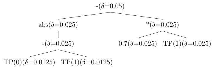
Without union bound optimization: each occurrence of the same variable uses a separate, smaller \(\delta\).

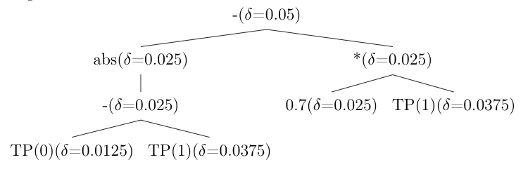
With union bound optimization: all occurrences share a combined \(\delta\), yielding tighter bounds.

uv run python -m fair_seldonian.experiments.runner bound

All Optimizations (opt)

Combines the modified confidence interval (Modified Confidence Interval (mod)), constant-aware delta allocation (Constant-Aware Delta Allocation (const)), and union bound optimization (Union Bound Optimization (bound)) for the tightest bounds.

uv run python -m fair_seldonian.experiments.runner opt

Lagrangian/KKT Optimization

An alternative candidate selection strategy based on Lagrangian relaxation [Boyd2004]. Rather than using the barrier-style penalty in the base algorithm, this approach formulates the constrained optimization as:

\[\mathcal{L}(\theta, \mu) = -f(\theta) + \mu \cdot \hat{g}(\theta)\]

where \(\mu \geq 0\) is the Lagrange multiplier.

Multiplier initialization. The value of \(\mu\) is estimated from the gradients of the objective and constraint at the initial (unconstrained) logistic regression solution \(\theta_0\):

\[\mu = \frac{-\nabla f(\theta_0)}{\nabla g(\theta_0)}\]

If the computed \(\mu\) is non-positive (indicating the constraint gradient does not oppose the objective gradient), it is set to 1.

Implementation details:

• The predict function returns probabilities (continuous in \([0, 1]\)) rather than discrete labels, enabling gradient computation.

• A single-pass approach is used: \(\mu\) is computed once from the initial solution, then the Lagrangian is minimized over \(\theta\) using the Powell optimizer. This avoids the computational cost of alternating optimization but may be less precise than iterative methods.

Note

This variant is experimental. The functions _get_cand_solution2 and _cand_obj2 in fair_seldonian.algorithms.qsa implement this approach but are not exposed in the public API.