Fair-Seldonian — Quickstart#

Fairness-constrained machine learning with high-confidence guarantees.

This notebook walks through the fair-seldonian package end to end:

Generate synthetic data with a controllable fairness gap
Train a model with the Quasi-Seldonian Algorithm (QSA)
Read the safety guarantee (passed + the high-confidence upper bound)
See the difference between a fair dataset (model returned) and an unfair one (No Solution Found)
Customise the constraint, confidence level $\delta$ , and inequality
Compare the five algorithm variants

The Seldonian guarantee: given a behavioural constraint and a confidence level $\delta$ , QSA either returns a model that satisfies the constraint with probability $\ge 1 - \delta$ , or it returns No Solution Found — it never returns an unsafe model.

0. Install#

Uncomment if the package isn’t already in your environment.

# %pip install fair-seldonian

import warnings

import matplotlib.pyplot as plt
import numpy as np
import torch

import fair_seldonian
from fair_seldonian.algorithms import QSA
from fair_seldonian.config import SeldonianConfig
from fair_seldonian.constraints.inequalities import Inequality
from fair_seldonian.data import data_split, get_data
from fair_seldonian.models import eval_ghat, predict, simple_logistic

warnings.filterwarnings("ignore")  # keep the demo output tidy

print("fair-seldonian version:", fair_seldonian.__version__)

fair-seldonian version: 3.1.0

1. The data#

get_data builds a synthetic binary-classification dataset where each row carries a sensitive attribute T $\in \{0, 1\}$ (e.g. a protected group).

argument	meaning
`N`	number of samples
`features`	number of feature columns
`t_ratio`	fraction of rows in group `T=1`
`tp0_ratio`	base positive-label rate for group `T=0`
`tp1_ratio`	base positive-label rate for group `T=1`
`random_seed`	reproducibility

The gap between tp0_ratio and tp1_ratio controls how unfair the underlying data is. data_split then returns train/test arrays as (X_test, Y_test, T_test, X_train, Y_train, T_train).

data = get_data(
    N=10000, features=5, t_ratio=0.4, tp0_ratio=0.4, tp1_ratio=0.6, random_seed=42
)
X_te, Y_te, T_te, X_tr, Y_tr, T_tr = data_split(
    frac=0.5, all_data=data, random_state=1, m_test=0.2
)

print("train:", X_tr.shape, " test:", X_te.shape)
print("group balance (train):", {g: int((T_tr == g).sum()) for g in (0, 1)})

train: (4000, 5)  test: (2000, 5)
group balance (train): {0: 2366, 1: 1634}

2. Train with QSA#

QSA(X, Y, T, seldonian_type, init_sol, init_sol1, config=DEFAULT_CONFIG)

Internally QSA splits the training data into a candidate set (used to find a solution) and a safety set (used to certify it). It returns a QSAResult with four fields:

theta, theta1 — the logistic-regression parameters (weights + bias)
passed_safety — True only if the candidate model passed the high-confidence safety test
diagnostics — why the run ended as it did. diagnostics.failure_mode distinguishes candidate_infeasible (no feasible model was found at all) from safety_test_rejected (one was found, but the safety data could not certify it). The two call for different remedies, so a bare “No Solution Found” hides the useful half of the answer.

Passing init_sol=None lets QSA warm-start from a plain logistic-regression fit. "opt" selects the variant with all confidence-bound optimisations enabled (see §6).

theta, theta1, passed, _ = QSA(X_tr, Y_tr, T_tr, "opt", None, None)

if passed:
    ub = float(eval_ghat(theta, theta1, X_te, Y_te, T_te, "opt"))
    print("Safety test PASSED \u2713")
    print(f"High-confidence upper bound on the constraint (test set): {ub:.4f}")
    print("A value \u2264 0 means the fairness constraint is satisfied.")
else:
    print(
        "No Solution Found \u2014 QSA refused to return a model it could not certify."
    )

No Solution Found — QSA refused to return a model it could not certify.

3. What is the constraint?#

Constraints are written in reverse-Polish (postfix) notation over per-group base variables.

There are two kinds, and the difference matters:

Cells — TP(g), FP(g), TN(g), FN(g) — are fractions of the whole group: TP(g) is $P(\hat{Y}=1, Y=1 \mid T=g)$ , a joint probability. The four cells sum to 1 within a group.
Rates — TPR(g), FPR(g), TNR(g), FNR(g) — condition on the label as well: TPR(g) is $P(\hat{Y}=1 \mid Y=1, T=g)$ , a mean over only that group’s positive rows, and so carries its own smaller sample size.
Predicted-positive / negative rates — PR(g) and NR(g), which are TP + FP and TN + FN. They ignore the label, so like the cells they are means over the whole group. Demographic parity written over PR costs two leaves rather than four.

The default constraint is:

TP(1) TP(0) - abs 0.25 TP(1) * -

which decodes to

g = \bigl|\, \mathrm{TP}(1) - \mathrm{TP}(0) \,\bigr| \; - \; 0.25 \cdot \mathrm{TP}(1)

so the gap in the joint true-positive cell must stay within 25 % of group 1’s. Note this is not equal opportunity, which compares true-positive rates; for that use TPR directly, or the ready-made builder equal_opportunity(epsilon). QSA certifies an upper confidence bound on $g$ rather than its point estimate — that is what makes the guarantee high-confidence.

def tp_rates(
    theta: torch.Tensor,
    theta1: torch.Tensor,
    X: np.ndarray,
    Y: np.ndarray,
    T: np.ndarray,
) -> dict[int, float]:
    """Empirical true-positive rate per group (for interpretation only)."""
    p = predict(theta, theta1, X).detach().numpy()
    yhat = (p >= 0.5).astype(int)
    rates: dict[int, float] = {}
    for g in (0, 1):
        mask = (T == g) & (Y == 1)
        rates[g] = float(yhat[mask].mean()) if mask.sum() else float("nan")
    return rates

4. Fair vs. unfair data#

The same algorithm behaves very differently depending on whether the constraint is achievable. We use the t-test inequality here, which gives tighter bounds than Hoeffding when the sample is reasonably large.

def run_scenario(name: str, tp0: float, tp1: float, config: SeldonianConfig) -> None:
    data = get_data(
        N=20000,
        features=5,
        t_ratio=0.5,
        tp0_ratio=tp0,
        tp1_ratio=tp1,
        random_seed=7,
    )
    X_te, Y_te, T_te, X_tr, Y_tr, T_tr = data_split(
        frac=1.0, all_data=data, random_state=1, m_test=0.3
    )
    theta, theta1, passed, _ = QSA(X_tr, Y_tr, T_tr, "opt", None, None, config)
    print(f"=== {name} ===")
    if passed:
        ub = float(eval_ghat(theta, theta1, X_te, Y_te, T_te, "opt", config))
        print(f"  PASSED \u2713   upper bound g = {ub:+.4f}  (\u2264 0 \u21d2 fair)")
        print(f"  test TP rates = {tp_rates(theta, theta1, X_te, Y_te, T_te)}")
    else:
        print("  No Solution Found \u2014 constraint could not be certified.")
    print()


cfg = SeldonianConfig(delta=0.05, inequality=Inequality.T_TEST)
run_scenario("Fair data  (tp0 = tp1 = 0.5)", 0.5, 0.5, cfg)
run_scenario("Unfair data (tp0 = 0.3, tp1 = 0.7)", 0.3, 0.7, cfg)

=== Fair data  (tp0 = tp1 = 0.5) ===
  PASSED ✓   upper bound g = -0.0438  (≤ 0 ⇒ fair)
  test TP rates = {0: 0.8553076402974983, 1: 0.8302488832163369}

=== Unfair data (tp0 = 0.3, tp1 = 0.7) ===
  PASSED ✓   upper bound g = -0.0037  (≤ 0 ⇒ fair)
  test TP rates = {0: 0.5568581477139508, 1: 0.22650602409638554}

With the default 25 % relative tolerance, both datasets certify — but look at what it costs. On the fair data the two groups’ true-positive rates come out close together and near the achievable ceiling. On the strongly unfair data QSA can only satisfy the constraint by suppressing predictions for the higher-base-rate group, which is visible in the lopsided TP rates: the model is dragged well away from the accuracy-maximising fit.

Refusal is still the behaviour that matters, and §5 shows it: tighten $\delta$ and the tolerance and QSA returns No Solution Found rather than a model it cannot prove is fair.

5. Custom configuration#

SeldonianConfig is a frozen dataclass:

field	default	meaning
`delta`	`0.05`	failure probability $\delta$ ; the guarantee holds w.p. $\ge 1-\delta$
`inequality`	`HOEFFDING_INEQUALITY`	confidence-bound method — see below
`constraint`	TP-gap constraint	postfix constraint string
`candidate_ratio`	`0.40`	fraction of training data used as the candidate set (rest is the safety set)
`optimizer`	`"Powell"`	any `method` accepted by `scipy.optimize.minimize`
`max_iter`	`10000`	iteration cap for candidate selection
`penalty`	`100.0`	weight on the constraint violation in the candidate objective

Four inequalities are available. HOEFFDING_INEQUALITY, EMPIRICAL_BERNSTEIN and BETTING are distribution-free and give a genuine high-confidence guarantee; T_TEST assumes approximate normality of the sample mean, which is what makes the result quasi-Seldonian. Empirical Bernstein and betting pay for the variance they measure rather than assuming the worst case of 1/4, so they are much tighter when a group’s rate is far from 1/2 — the common case for a minority group. Betting is the tightest and the slowest.

Below: a stricter confidence level ( $\delta = 0.01$ ) and a tighter constraint — the gap must stay within 15 % of group 1’s cell (vs. 25 % by default).

strict = SeldonianConfig(
    delta=0.01,
    inequality=Inequality.T_TEST,
    constraint="TP(1) TP(0) - abs 0.15 TP(1) * -",
    candidate_ratio=0.5,
)
run_scenario("Strict (\u03b4=0.01, 15% gap)", 0.5, 0.5, strict)

=== Strict (δ=0.01, 15% gap) ===
  No Solution Found — constraint could not be certified.

6. Algorithm variants#

The seldonian_type string selects how the confidence interval is constructed. Tighter bounds make it easier to certify a fair model on a given amount of data.

Mode	Description
`base`	Standard Hoeffding bound, uniform $\delta$ -splitting
`mod`	Decomposed candidate/safety estimation error
`const`	Constant-aware $\delta$ allocation
`bound`	Union-bound optimisation for repeated variables
`opt`	All optimisations combined
`affine`	Compiles the constraint to a max of affine forms and bounds each with a single interval, exploiting the independence of disjoint groups. Roughly halves the slack, but only applies to constraints built from `+`, `-`, scaling by a constant and `abs`; anything else raises `NotAffine`.

We run each variant on the same fair dataset and compare the certified upper bound (lower = tighter).

data = get_data(
    N=20000, features=5, t_ratio=0.5, tp0_ratio=0.5, tp1_ratio=0.5, random_seed=7
)
X_te, Y_te, T_te, X_tr, Y_tr, T_tr = data_split(
    frac=1.0, all_data=data, random_state=1, m_test=0.3
)
cfg = SeldonianConfig(delta=0.05, inequality=Inequality.T_TEST)

print(f"{'mode':>6} | {'passed':>6} | upper bound g (test)")
print("-" * 40)
for mode in ("base", "mod", "const", "bound", "opt"):
    theta, theta1, passed, _ = QSA(X_tr, Y_tr, T_tr, mode, None, None, cfg)
    ub = float(eval_ghat(theta, theta1, X_te, Y_te, T_te, mode, cfg))
    print(f"{mode:>6} | {str(passed):>6} | {ub:+.4f}")

  mode | passed | upper bound g (test)
----------------------------------------
  base |   True | -0.0402
   mod |   True | -0.0402
 const |   True | -0.0408
 bound |   True | -0.0422

   opt |   True | -0.0438

7. With vs. without QSA — the price and value of the guarantee#

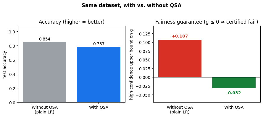
The clearest way to see what QSA buys you is to run the same dataset through two models:

Without QSA — plain logistic regression (simple_logistic), which only maximises accuracy.
With QSA — the Seldonian algorithm, which maximises accuracy subject to the fairness constraint holding with high confidence.

We compare test accuracy and the high-confidence upper bound on the constraint $g$ (the same quantity eval_ghat returns). Plain logistic regression is a few points more accurate, but its bound sits above zero — on this data its fairness cannot be certified. QSA trades a little accuracy for a certified guarantee ( $g \le 0$ ). That trade — a small, explicit accuracy cost in exchange for a provable safety guarantee — is the whole point of the Seldonian approach.

# Same dataset for both models. get_data seeds its own generator
# from random_seed, so the draw is reproducible without touching
# the global NumPy RNG.
cmp_data = get_data(
    N=20000, features=5, t_ratio=0.5, tp0_ratio=0.4, tp1_ratio=0.6, random_seed=7
)
Xc_te, Yc_te, Tc_te, Xc_tr, Yc_tr, Tc_tr = data_split(
    frac=1.0, all_data=cmp_data, random_state=1, m_test=0.3
)
cmp_cfg = SeldonianConfig(delta=0.05, inequality=Inequality.T_TEST)


def accuracy(
    theta: torch.Tensor, theta1: torch.Tensor, X: np.ndarray, Y: np.ndarray
) -> float:
    yhat = (predict(theta, theta1, X).detach().numpy() >= 0.5).astype(int)
    return float((yhat == Y).mean())


# Without QSA: plain logistic regression, no fairness constraint.
lr_theta, lr_theta1 = simple_logistic(Xc_tr, Yc_tr)
lr_acc = accuracy(lr_theta, lr_theta1, Xc_te, Yc_te)
lr_bound = float(eval_ghat(lr_theta, lr_theta1, Xc_te, Yc_te, Tc_te, "opt", cmp_cfg))

# With QSA: same data, fairness constraint enforced with high confidence.
qsa_theta, qsa_theta1, qsa_passed, _ = QSA(
    Xc_tr, Yc_tr, Tc_tr, "opt", None, None, cmp_cfg
)
qsa_acc = accuracy(qsa_theta, qsa_theta1, Xc_te, Yc_te)
qsa_bound = float(eval_ghat(qsa_theta, qsa_theta1, Xc_te, Yc_te, Tc_te, "opt", cmp_cfg))

for name, acc, bound in [
    ("Without QSA", lr_acc, lr_bound),
    ("With QSA   ", qsa_acc, qsa_bound),
]:
    verdict = "certified fair" if bound <= 0 else "NOT certifiable"
    print(f"{name}: accuracy={acc:.3f}  bound g={bound:+.3f}  → {verdict}")

labels = ["Without QSA\n(plain LR)", "With QSA"]
accs = [lr_acc, qsa_acc]
bounds = [lr_bound, qsa_bound]

fig, (ax1, ax2) = plt.subplots(1, 2, figsize=(9, 4))

ax1.bar(labels, accs, color=["#9aa0a6", "#1a73e8"])
ax1.set_ylim(0, 1.08)
ax1.set_ylabel("test accuracy")
ax1.set_title("Accuracy (higher = better)")
for i, v in enumerate(accs):
    ax1.annotate(
        f"{v:.3f}", (i, v), textcoords="offset points", xytext=(0, 4), ha="center"
    )

bar_colors = ["#d93025" if b > 0 else "#188038" for b in bounds]
ax2.bar(labels, bounds, color=bar_colors)
ax2.axhline(0, color="black", linewidth=1)
pad = 0.04
ax2.set_ylim(min(bounds) - pad, max(bounds) + pad)
ax2.set_ylabel("high-confidence upper bound on g")
ax2.set_title("Fairness guarantee (g ≤ 0 ⇒ certified fair)")
for i, v in enumerate(bounds):
    ax2.annotate(
        f"{v:+.3f}",
        (i, v),
        textcoords="offset points",
        xytext=(0, 6 if v >= 0 else -14),
        ha="center",
        fontweight="bold",
        color=bar_colors[i],
    )

fig.suptitle("Same dataset, with vs. without QSA", fontweight="bold")
fig.tight_layout(rect=[0, 0, 1, 0.96])
plt.show()

Without QSA: accuracy=0.854  bound g=+0.107  → NOT certifiable
With QSA   : accuracy=0.787  bound g=-0.032  → certified fair

../_images/deab0b9a65891c5aee8795ca5786e83ef922294a142bfc1846237540b9d475e0.png

Next steps#

Swap in your own data: arrange features as X, binary labels as Y, and a binary sensitive attribute as T (all NumPy arrays), then call QSA(X, Y, T, "opt", None, None, config).
Write your own constraint in postfix form over the cells TP/FP/TN/FN(group) and the rates TPR/FPR/TNR/FNR(group) — or start from a builder such as demographic_parity, equal_opportunity or equalized_odds.
Read the docs: https://parulgupta1004.github.io/fair-seldonian/