Fair-Seldonian on real data: UCI Adult income#

This notebook applies the Quasi-Seldonian Algorithm (QSA) to the UCI Adult income dataset under a demographic-parity constraint, and shows both sides of the Seldonian guarantee on real data:

an ordinary logistic regression reaches good accuracy but predicts the positive class at very different rates for the two groups (a demographic-parity gap), and
QSA, asked to certify that gap is bounded, returns No Solution Found rather than shipping the biased model.

Task framing

symbol	meaning
`Y` (label)	income > 50K
`T` (sensitive)	sex (1 = Male, 0 = Female)
`X` (features)	standardized numeric columns, with `T` appended as the final column (library convention)

Requires network access on the first run to download the dataset (cached afterwards).

Background: what is demographic parity?#

Demographic parity (also called statistical parity or the independence criterion) asks that a model’s prediction be statistically independent of the sensitive attribute. For a binary classifier with prediction $\hat{Y}$ and sensitive group $A$ :

P(\hat{Y} = 1 \mid A = a) = P(\hat{Y} = 1 \mid A = b) \quad \text{for all groups } a, b.

In words: every group is predicted positive at the same rate, regardless of the true label $Y$ . In practice we bound the gap by a tolerance $\epsilon$ :

\left| P(\hat{Y}=1 \mid A=1) - P(\hat{Y}=1 \mid A=0) \right| \le \epsilon,

which is exactly what we enforce below with $\epsilon = 0.10$ . A closely related industry rule of thumb is the disparate-impact “four-fifths (80%) rule”, which compares the ratio of group positive rates rather than their difference (Feldman et al., 2015).

How it differs from equalized opportunity. Because demographic parity ignores $Y$ , it can be met by a model that is deliberately inaccurate for one group. Label-conditioned criteria such as equalized odds and equalized opportunity (Hardt et al., 2016) instead require error rates to match across groups. There is no single “correct” fairness metric: the appropriate choice is context-dependent, and several criteria are provably incompatible except in degenerate cases (Barocas, Hardt & Narayanan, 2023; Dwork et al., 2012).

Why demographic parity for this task? Predicting income > 50K stands in here for an allocative decision - one where a positive prediction grants access to a benefit (a loan, an interview, a targeted offer). When the goal is equal access across groups, demographic parity is a natural target: it constrains the rate at which the benefit is allocated to each group. This is especially appropriate for Adult, where the labels themselves reflect historical disparities (men are labelled high-income far more often), so a label-conditioned criterion would bake that societal gap in as ground truth. If instead you trusted the labels and only wanted equal accuracy among the truly-qualified, equalized opportunity would fit better (see custom_constraint.py).

In this library, the predicted-positive rate is the base variable PR(g), so demographic parity is written as the postfix constraint PR(1) PR(0) - abs 0.1 -. The builder demographic_parity(epsilon) produces exactly that, which is what we use below.

PR(g) is equivalent to TP(g) + FP(g) — the confusion-matrix cells are fractions of each group and sum to 1 within it — but writing it as one base variable rather than two matters for the bound. Every leaf of the constraint spends its own slice of $\delta$ , so the two-leaf form is certifiable at a tighter $\epsilon$ than the four-leaf one: on this data, 0.15 against 0.20.

import numpy as np
from sklearn.datasets import fetch_openml

from fair_seldonian.algorithms import QSA
from fair_seldonian.config import SeldonianConfig
from fair_seldonian.models import predict, simple_logistic

1. Load and frame the data#

We download Adult, derive the binary label and sensitive attribute, standardize the numeric features, and append the sensitive attribute as the final feature column. Then we take a deterministic subsample and train/test split.

frame = fetch_openml("adult", version=2, as_frame=True, parser="auto").frame.dropna()

T = (frame["sex"].astype(str) == "Male").astype(int).to_numpy()
Y = frame["class"].astype(str).str.contains(">50K").astype(int).to_numpy()

numeric = frame.select_dtypes("number")
standardized = (numeric - numeric.mean()) / numeric.std()
X = np.column_stack([standardized.to_numpy(), T]).astype(float)

# deterministic subsample + split for a fast, reproducible demo
rng = np.random.default_rng(0)
idx = rng.permutation(len(X))[:8000]
X, Y, T = X[idx], Y[idx], T[idx]
cut = int(0.7 * len(X))
X_tr, Y_tr, T_tr = X[:cut], Y[:cut], T[:cut]
X_te, Y_te, T_te = X[cut:], Y[cut:], T[cut:]

print(
    f"Adult: {len(X)} examples, positive rate {Y.mean():.3f}, male share {T.mean():.3f}"
)

Adult: 8000 examples, positive rate 0.241, male share 0.678

2. Unconstrained baseline#

A plain logistic regression. We measure overall accuracy and the predicted-positive rate within each group; the gap between those rates is the demographic-parity violation the fairness constraint targets.

def positive_rate(pred, mask):
    # P(pred = 1 | T = group): the predicted-positive rate for a group
    return float(pred[mask].mean()) if mask.any() else float("nan")


theta, theta1 = simple_logistic(X_tr, Y_tr)
pred = (predict(theta, theta1, X_te).detach().numpy() >= 0.5).astype(int)

acc = float((pred == Y_te).mean())
pr_male = positive_rate(pred, T_te == 1)
pr_female = positive_rate(pred, T_te == 0)
dp_gap = abs(pr_male - pr_female)

print(f"accuracy               : {acc:.3f}")
print(f"positive rate (male)   : {pr_male:.3f}")
print(f"positive rate (female) : {pr_female:.3f}")
print(f"demographic-parity gap : {dp_gap:.3f}")

accuracy               : 0.814
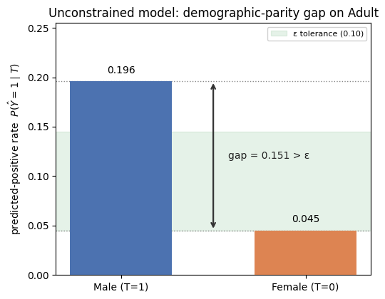
positive rate (male)   : 0.196
positive rate (female) : 0.045
demographic-parity gap : 0.151

The bars below show that gap directly. The male predicted-positive rate clears the $\epsilon$ tolerance band drawn around the (lower) female rate, so the demographic-parity constraint is violated - which is exactly why QSA declines to certify this model in the next section.

# Visualize the demographic-parity gap measured on the test set above: each
# group's predicted-positive rate, with the epsilon tolerance band drawn up from
# the lower rate. The constraint is violated when the other bar clears the band.
import matplotlib.pyplot as plt

eps = 0.10  # the tolerance enforced by the fairness constraint below
rates = [pr_male, pr_female]
labels = ["Male (T=1)", "Female (T=0)"]
colors = ["#4C72B0", "#DD8452"]
lo, hi = min(rates), max(rates)

fig, ax = plt.subplots(figsize=(5.4, 4.3))
ax.axhspan(
    lo,
    lo + eps,
    color="#55A868",
    alpha=0.15,
    zorder=1,
    label=f"\u03b5 tolerance ({eps:.2f})",
)
ax.axhline(lo, ls=":", color="#888888", lw=1, zorder=2)
ax.axhline(hi, ls=":", color="#888888", lw=1, zorder=2)

bars = ax.bar(labels, rates, color=colors, width=0.55, zorder=3)
for bar, rate in zip(bars, rates):
    ax.text(
        bar.get_x() + bar.get_width() / 2,
        rate + 0.006,
        f"{rate:.3f}",
        ha="center",
        va="bottom",
        fontsize=10,
    )

# gap arrow drawn in the empty space between the two bars
ax.annotate(
    "",
    xy=(0.5, hi),
    xytext=(0.5, lo),
    arrowprops=dict(arrowstyle="<->", color="#333333", lw=1.6),
)
ax.text(
    0.58,
    (lo + hi) / 2,
    f"gap = {dp_gap:.3f} > \u03b5",
    va="center",
    ha="left",
    fontsize=10,
    color="#222222",
)

ax.set_ylim(0, max(rates) * 1.3)
ax.set_ylabel(r"predicted-positive rate  $P(\hat{Y}=1 \mid T)$")
ax.set_title("Unconstrained model: demographic-parity gap on Adult", fontsize=12)
ax.legend(loc="upper right", fontsize=8, framealpha=0.9)
fig.tight_layout()
plt.show()

../_images/0bfacc133101f96d3569b513160714fa4e03f74c661b0292639206fb400aa926.png

3. The Seldonian guarantee (demographic parity)#

Now we ask QSA to return a model only if it can certify the demographic-parity constraint holds with high probability. On this data it declines.

from fair_seldonian import demographic_parity

# Demographic parity at a 10-point tolerance: PR(1) PR(0) - abs 0.1 -
config = SeldonianConfig(constraint=demographic_parity(0.10))
result = QSA(X_tr, Y_tr, T_tr, "opt", None, None, config)

if result.passed_safety:
    print("certified: demographic parity holds with high confidence")
else:
    print("No Solution Found - QSA will not certify demographic parity here,")
    print("rather than return a model with the disparity shown above.")
    print(f"  reason: {result.diagnostics.failure_mode}")

No Solution Found - QSA will not certify demographic parity here,
rather than return a model with the disparity shown above.
  reason: safety_test_rejected

4. What would certify, and what it costs#

Refusing is only half an answer. The unconstrained gap is 0.151, so no model can meet a tolerance below that without changing its predictions — the question is how much tolerance is needed, and what accuracy is surrendered to get it.

Adult is 24.1% positive, so a model that predicts nobody earns over 50K scores about 0.76 — the exact figure for this test split is printed below. That is the number to judge the certified models against: anything below it is worse than a constant.

baseline_acc = float(max(Y_te.mean(), 1 - Y_te.mean()))
sweep = []  # (epsilon, certified, accuracy, gap) - reused by the chart below

print(f"{'epsilon':>8} {'verdict':>22} {'accuracy':>9} {'gap':>7}")
print("-" * 50)
for eps in (0.10, 0.15, 0.20, 0.30):
    r = QSA(
        X_tr,
        Y_tr,
        T_tr,
        "opt",
        None,
        None,
        SeldonianConfig(constraint=demographic_parity(eps)),
    )
    if r.passed_safety:
        p = (predict(r.theta, r.theta1, X_te).detach().numpy() >= 0.5).astype(int)
        model_acc = float((p == Y_te).mean())
        model_gap = abs(float(p[T_te == 1].mean()) - float(p[T_te == 0].mean()))
        sweep.append((eps, True, model_acc, model_gap))
        print(f"{eps:>8.2f} {'certified':>22} {model_acc:>9.3f} {model_gap:>7.3f}")
    else:
        sweep.append((eps, False, None, None))
        print(f"{eps:>8.2f} {r.diagnostics.failure_mode:>22} {'-':>9} {'-':>7}")
print(f"\nunconstrained : accuracy {acc:.3f}, gap {dp_gap:.3f}")
print(f"predict-nobody: accuracy {baseline_acc:.3f}, gap 0.000")

 epsilon                verdict  accuracy     gap
--------------------------------------------------
    0.10   safety_test_rejected         -       -

    0.15              certified     0.479   0.069

    0.20              certified     0.697   0.064

    0.30              certified     0.760   0.126

unconstrained : accuracy 0.814, gap 0.151
predict-nobody: accuracy 0.765, gap 0.000

# Two panels sharing the epsilon axis. Accuracy and the parity gap are different
# measures, so they get their own axes rather than being crushed onto one plot
# with two y-scales.
SURFACE, GRID = "#fcfcfb", "#e1e0d9"
INK, MUTED = "#0b0b0b", "#898781"
CERTIFIED, REFUSED = "#2a78d6", "#eb6834"  # validated categorical slots 1 and 2

eps_all = [e for e, *_ in sweep]
ok = [(e, a, g) for e, c, a, g in sweep if c]
refused_upto = max([e for e, c, *_ in sweep if not c], default=None)

fig, (ax_acc, ax_gap) = plt.subplots(
    1, 2, figsize=(10.5, 4.0), sharex=True, facecolor=SURFACE
)
for ax in (ax_acc, ax_gap):
    ax.set_facecolor(SURFACE)
    ax.grid(True, color=GRID, linewidth=0.8, zorder=0)
    ax.set_axisbelow(True)
    for side in ("top", "right"):
        ax.spines[side].set_visible(False)
    for side in ("left", "bottom"):
        ax.spines[side].set_color("#c3c2b7")
    ax.tick_params(colors=MUTED, labelsize=9)
    ax.set_xlabel(r"tolerance $\epsilon$", color=MUTED, fontsize=10)
    if refused_upto is not None:
        # Everything at or below this epsilon was refused: there is no model to
        # plot, so the region is shaded rather than given a fabricated point.
        ax.axvspan(
            min(eps_all) - 0.02,
            (refused_upto + 0.15) / 2,
            color=REFUSED,
            alpha=0.10,
            zorder=1,
            label="no solution found",
        )

ax_acc.plot(
    [e for e, *_ in ok],
    [a for _, a, _ in ok],
    "-o",
    color=CERTIFIED,
    linewidth=2,
    markersize=8,
    zorder=3,
    label="certified model",
)
ax_acc.axhline(acc, ls="--", lw=1.2, color=MUTED, zorder=2)
ax_acc.axhline(baseline_acc, ls="--", lw=1.2, color=MUTED, zorder=2)
ax_acc.text(
    0.084, acc, "unconstrained", va="bottom", ha="left", fontsize=8, color=MUTED
)
ax_acc.text(
    0.084,
    baseline_acc,
    "predict nobody",
    va="bottom",
    ha="left",
    fontsize=8,
    color=MUTED,
)
# Direct-label only the point that carries the argument, and the endpoint.
for e, a, _ in (ok[0], ok[-1]):
    ax_acc.annotate(
        f"{a:.3f}",
        (e, a),
        textcoords="offset points",
        xytext=(0, -16),
        ha="center",
        fontsize=9,
        color=INK,
    )
ax_acc.set_ylabel("accuracy on held-out data", color=MUTED, fontsize=10)
ax_acc.set_ylim(0.40, 0.90)
ax_acc.set_title(
    "Certified, but is it useful?",
    color=INK,
    fontsize=11,
    fontweight="bold",
    loc="left",
)

ax_gap.plot(
    [e for e, *_ in ok],
    [g for _, _, g in ok],
    "-o",
    color=CERTIFIED,
    linewidth=2,
    markersize=8,
    zorder=3,
    label="certified model",
)
ax_gap.plot(eps_all, eps_all, ls="--", lw=1.2, color=MUTED, zorder=2)
ax_gap.axhline(dp_gap, ls="--", lw=1.2, color=MUTED, zorder=2)
ax_gap.text(
    0.084, dp_gap, "unconstrained", va="bottom", ha="left", fontsize=8, color=MUTED
)
ax_gap.text(
    0.263,
    0.290,
    r"gap = $\epsilon$",
    fontsize=8,
    color=MUTED,
    rotation=30,
    rotation_mode="anchor",
)
ax_gap.set_ylabel("demographic-parity gap", color=MUTED, fontsize=10)
ax_gap.set_ylim(0, 0.34)
ax_gap.set_title(
    "The gap it actually achieves",
    color=INK,
    fontsize=11,
    fontweight="bold",
    loc="left",
)

ax_acc.legend(loc="lower right", fontsize=8, framealpha=0.9)
fig.tight_layout()
plt.show()

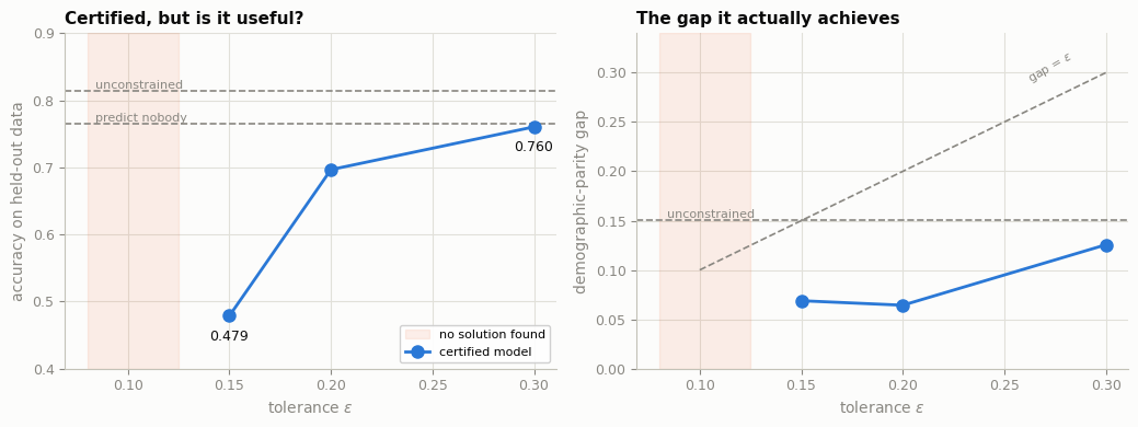
../_images/7efca94b0d606f1fd382180b622928be1564de49dd81ded98771662ffed97cce.png

Two things stand out. Certification arrives at $\epsilon = 0.15$ , but the model that achieves it scores 0.479 — well below the predict-nobody baseline, so it is certified and useless. Only by $\epsilon = 0.30$ does accuracy recover to roughly the constant-model level, and by then the tolerated gap is 0.30, twice the disparity we started with.

At $\epsilon = 0.10$ the refusal is safety_test_rejected rather than candidate_infeasible: candidate selection did find a model satisfying the constraint, and the safety set declined to certify it. That is the mode that says more data would help, as against the constraint being unreachable.

The honest reading is that demographic parity is expensive on Adult at any tolerance worth having — which is a result about the data and the criterion, not a defect in the algorithm.

Takeaway#

The unconstrained model is accurate but predicts high income far more often for one group than the other. QSA trades coverage for safety: on data where it cannot prove demographic parity holds, it returns no model at all - never an unsafe one. See quickstart.ipynb for cases where QSA does certify, and custom_constraint.py for other fairness definitions.

References#

Seldonian algorithms

Thomas, P. S., da Silva, B. C., Barto, A. G., Giguère, S., Brun, Y., & Brunskill, E. (2019). Preventing undesirable behavior of intelligent machines. Science, 366(6468), 999-1004. https://doi.org/10.1126/science.aag3311

Demographic parity and fairness criteria

Dwork, C., Hardt, M., Pitassi, T., Reingold, O., & Zemel, R. (2012). Fairness through awareness. ITCS ‘12, 214-226. https://arxiv.org/abs/1104.3913
Feldman, M., Friedler, S. A., Moeller, J., Scheidegger, C., & Venkatasubramanian, S. (2015). Certifying and removing disparate impact. KDD ‘15. https://arxiv.org/abs/1412.3756
Hardt, M., Price, E., & Srebro, N. (2016). Equality of opportunity in supervised learning. NeurIPS 2016. https://arxiv.org/abs/1610.02413
Barocas, S., Hardt, M., & Narayanan, A. (2023). Fairness and Machine Learning: Limitations and Opportunities. MIT Press. https://fairmlbook.org

Dataset

Becker, B., & Kohavi, R. (1996). Adult [Dataset]. UCI Machine Learning Repository. https://doi.org/10.24432/C5XW20
Kohavi, R. (1996). Scaling up the accuracy of naive-Bayes classifiers: a decision-tree hybrid. KDD ‘96, 202-207. https://cdn.aaai.org/KDD/1996/KDD96-033.pdf