Concentration Inequalities

Every bound in the framework rests on a confidence interval for the mean of a base variable. Which inequality builds that interval is set on the configuration and is orthogonal to the seldonian_type variant: Algorithm Variants decides how the intervals are combined, the inequality decides how wide each one is.

from fair_seldonian import Inequality, SeldonianConfig

config = SeldonianConfig(inequality=Inequality.EMPIRICAL_BERNSTEIN)

Inequality	Assumption	Guarantee	Half-width at n=2000, rate 0.1
T_TEST	the sample mean is approximately normal	asymptotic only	0.0131
HOEFFDING_INEQUALITY	each term lies in [0, 1]	distribution-free	0.0304
EMPIRICAL_BERNSTEIN	each term lies in [0, 1]	distribution-free	0.0225
BETTING	each term lies in [0, 1]	distribution-free	0.0142

The final column is not a quoted figure: it is computed at build time by running each implementation on one fixed Bernoulli sample, so the ordering shown is the ordering the library actually delivers. At a base rate of 0.1 the three distribution-free options rank betting < empirical Bernstein < Hoeffding, which is the ranking the sections below explain. Student’s t is narrower still, but see the warning against relying on it.

The first three are distribution-free: they assume only that each contribution lies in $[0, 1]$, which the base variables satisfy by construction. Their coverage claim holds at any sample size.

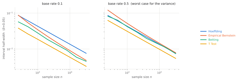
Half-width against sample size, averaged over 15 draws. Produced by scripts/make_docs_figures.py calling the same implementations the library uses, so it cannot disagree with them.

The two panels are the whole argument for offering a choice. At a base rate of 0.1 the ordering is betting < empirical Bernstein < Hoeffding, and the gap is large: betting is worth roughly a four-fold increase in sample size over Hoeffding, since a half-width scales as $1/\sqrt{n}$. At 0.5 empirical Bernstein crosses above Hoeffding — it has paid the additive variance-estimation term for a variance that was already the worst case — while betting converges onto Hoeffding.

Which to use

Start here

HOEFFDING_INEQUALITY

Cheap, predictable, and never worse than a constant factor off. Nothing about it depends on the data, so it cannot surprise you.

A group’s rate is small

EMPIRICAL_BERNSTEIN

Any rate far from 1/2 — the usual case for a minority group, or for a constraint on a rare error. Avoid it when the rate really is near 1/2.

The bound is what blocks you

BETTING

Tightest of the three sound options at every rate. Pay for it in time: each endpoint takes repeated passes over the data.

Note

Because these are orthogonal to Algorithm Variants, changing inequality costs one argument and never changes what is being certified — only how much slack the certificate carries. examples/tighter_bounds.py prints the full grid.

Hoeffding (HOEFFDING_INEQUALITY)

The default. For a mean of $n$ i.i.d. terms in $[0, 1]$ [Hoeffding1963]:

$$\text{half-width} = \sqrt{\frac{\ln(c/\delta)}{2n}}$$

where $c = 2$ for a two-sided interval and $c = 1$ for a one-sided one. A symmetric interval fails if either side is breached, so the budget must be split between them; using $\ln(1/\delta)$ two-sided would deliver coverage $1 - 2\delta$, not $1 - \delta$.

Hoeffding assumes the worst possible variance, $1/4$. That is exactly right for a base rate of $1/2$ and increasingly pessimistic away from it.

Empirical Bernstein (EMPIRICAL_BERNSTEIN)

Pays for the variance it measures rather than the worst case [MaurerPontil2009]:

$$\text{half-width} = \sqrt{\frac{2\hat{\sigma}^2 \ln(c/\delta)}{n}} + \frac{7\ln(c/\delta)}{3(n-1)}$$

with $\hat{\sigma}^2$ the unbiased sample variance. The additive second term is the price of estimating the variance from the same sample.

When it wins. Tighter than Hoeffding whenever $\hat{\sigma}^2 < 1/4$, and slightly looser at exactly $1/2$, where the additive term is paid for nothing. Since a group’s rate being small is the common case for a minority group, this is often the better default in practice.

Betting (BETTING)

The Waudby-Smith and Ramdas betting interval [WaudbySmith2024]. Two nonnegative martingales are run against each candidate mean $m$ — one betting the true mean exceeds $m$, one that it falls below. Under the hypothesis each has unit expectation, so by Ville’s inequality [Ville1939] each exceeds $2/\delta$ with probability at most $\delta/2$. Rejecting when either does gives a level-$\delta$ test, and inverting that test over $m$ gives the interval.

The bets must be predictable — a function of $x_1, \dots, x_{i-1}$ only — or the martingale property fails and the guarantee with it. They are therefore computed from a running mean and variance that exclude the current observation.

Trade-off. It adapts to the observed variance like empirical Bernstein but without paying the additive penalty term, so it dominates both other sound options for bounded variables. The cost is compute: the interval is found by anchoring at the sample mean, walking outwards until the test rejects, and bisecting, with each step a pass over the data.

Student’s t (T_TEST)

Warning

This is the one option that does not give a genuine high-confidence guarantee. It is what puts the quasi in quasi-Seldonian.

$$\text{half-width} = \frac{\hat{\sigma}}{\sqrt{n}}\, t_{1-\delta/c,\; n-1}$$

Student’s t interval [Student1908] assumes the sample mean is approximately normal. That is an appeal to the central limit theorem, not a finite-sample bound, so the guarantee is only as good as the approximation. It is included because [Thomas2019] uses it and comparisons against the published results need it; prefer one of the three above for any claim that has to hold.

Measuring the failure rate (clopper_pearson)

The four above bound a constraint inside the algorithm. A separate question is whether the algorithm delivered on its promise: across repeated trials, how often did a returned model actually violate the constraint? That rate should sit at or below $\delta$.

clopper_pearson() puts an exact binomial interval [ClopperPearson1934] on that count. Exactness matters here: the interesting outcome is usually zero observed violations, and a normal approximation collapses to the degenerate interval $[0, 0]$ — claiming certainty from evidence that supports nothing of the kind. The exact interval instead reports $[0,\, 1 - (\delta_{\text{tail}})^{1/n}]$, which shrinks with $n$ but never reaches zero.

from fair_seldonian import clopper_pearson

lo, hi = clopper_pearson(successes=0, n=200, alpha=0.05)

Seeing the difference

examples/tighter_bounds.py certifies one fixed model under every combination of seldonian_type and inequality, printing the resulting bound so the slack attributable to each choice is visible side by side:

uv run python examples/tighter_bounds.py